> For the complete documentation index, see [llms.txt](https://docs.nimbusimage.com/llms.txt). Markdown versions of documentation pages are available by appending `.md` to page URLs; this page is available as [Markdown](https://docs.nimbusimage.com/documentation/viewing-your-data.md).

# Viewing your image dataset

Once your images are loaded into NimbusImage, you can interact with it through the viewer. The viewer allows for easy navigation and flexible visualization.

**Key features include:**

* **Easy to use navigation and contrast settings**
* **"Unrolling" of variables** to show montages
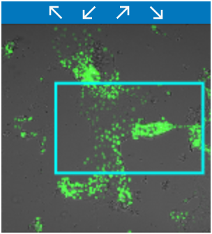
* **Overview "minimap".** Drag around the square to navigate; shift-click-drag to directly go to a location.

  <figure><img src="/files/UXIyzora4GvC1XaKajyE" alt="" width="156"><figcaption></figcaption></figure>
* **Dynamic scale bar.** Click the scale bar to adjust pixel sizes and other settings.
* **Zoom in and out of large images.** Scroll wheel zooms, just like Google Maps.
* **Flexible layer settings.** See below for more information about layers.

## Layers

Understanding layers can help unlock more flexibility in how you visualize your data. Generally, layers are most commonly thought of as mapping to channels, but in NimbusImage, they are capable of more. For instance, you can make multiple layers that draw from the same channel, but show different times in different colors, which can be very helpful for time lapse analysis.

<figure><img src="/files/kvBR6BLA7oAdBA1Ha6H6" alt=""><figcaption><p>Current time in green, next time in red so that you can see the shift</p></figcaption></figure>

### Layer grouping

Another useful feature is layer grouping, which allows you to put together multiple layers into a single grouped layer. For instance, if you have a couple fluorescence channels that you always want to show together, you can group them.

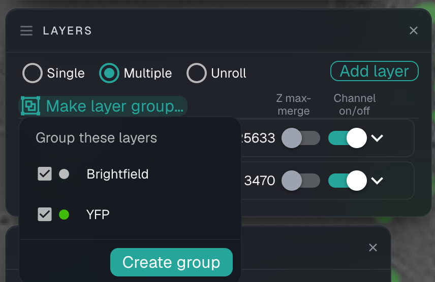
To create a group, click **"Make layer group…"** at the top of the Layers panel, check the layers you want to combine, and click **Create group**:

<figure><img src="/files/SU8CryUwHCn4boLIOrrO" alt=""><figcaption></figcaption></figure>

You can group any number of layers together, and ungroup them later from the group's menu.

## Label display options

NimbusImage allows you to customize how labels are displayed in your image viewer. You can toggle between:

* **Text labels**: Display descriptive labels such as "Well A1", "Position 3", etc.
* **Numeric identifiers**: Display simple numeric IDs for a cleaner view

This toggle helps you choose between more informative labels and a less cluttered display depending on your needs.

## Custom channel color preferences

You can set default channel color preferences in your user profile. These custom color settings:

* Automatically apply to new datasets you create or upload
* Can be overridden on a per-dataset basis if you want different colors for a specific dataset
* Help maintain consistency across your analyses

This feature is especially useful if you work with the same types of channels regularly and want them to always appear in your preferred colors.

## 3D visualization

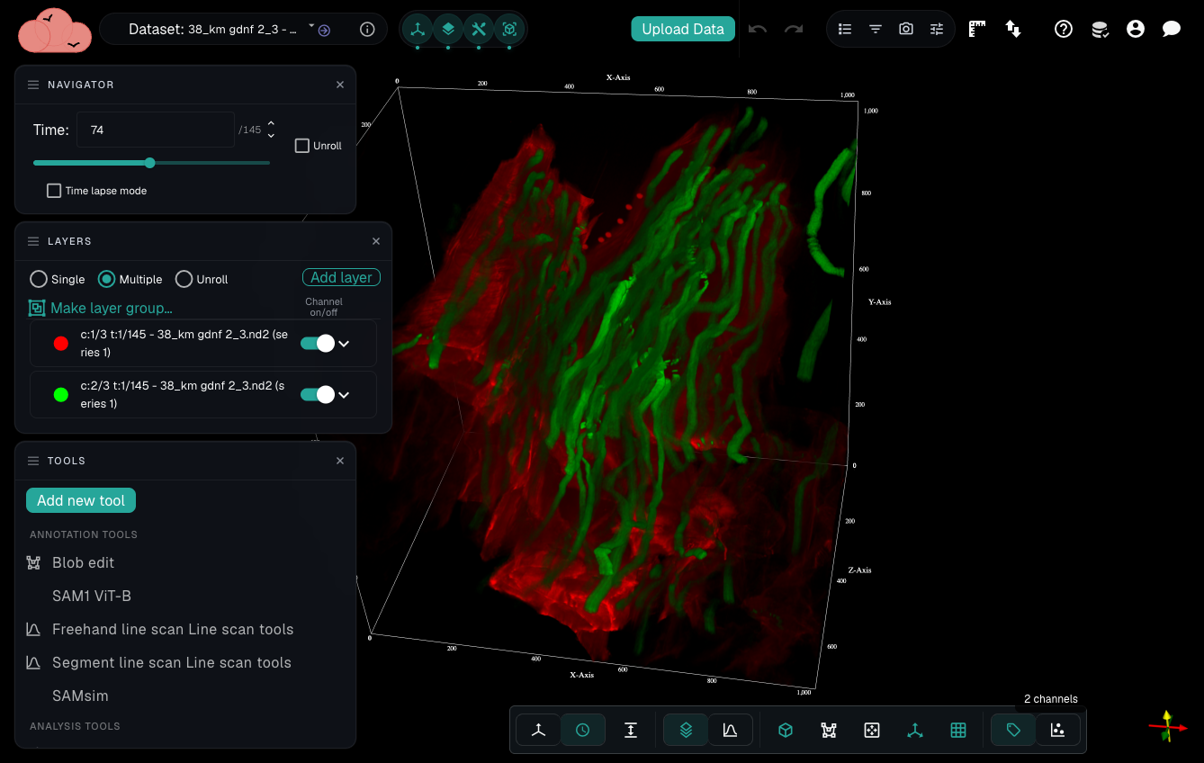
In addition to the standard 2D viewer, NimbusImage can render your dataset as an interactive 3D volume directly in your browser. This is useful for exploring Z-stacks and for viewing time lapses as volumes. Toggle between the 2D and 3D views using the control in the top app bar.

<figure><img src="/files/xYK6q0Fden8ds8xSf6Xz" alt=""><figcaption><p>A time lapse rendered in 3D with Time mapped to the depth axis: each green streak is a nucleus tracing its path (a "worldline") over time. The scaled bounding box and 3D controls run along the edges.</p></figcaption></figure>

### Volume rendering

Each layer is volume-rendered using the same color and contrast settings you use in the 2D viewer. Two blend modes are available:

* **Composite**: Blends all channels together, so overlapping structures appear semi-transparent.
* **Maximum Intensity Projection (MIP)**: Shows the brightest value along each viewing ray, which is useful for emphasizing bright puncta or fibers.

The volume respects anisotropic voxel spacing (the physical Z-step relative to the XY pixel size), so structures keep their true proportions.

{% hint style="info" %}
Very large images are automatically downsampled to stay within your browser's memory and GPU limits. This affects only the 3D preview, not your underlying data.
{% endhint %}

### Choosing the depth axis: Z or Time

You can map either **Z** or **Time** to the depth axis of the volume:

* Use **Z** to view a conventional Z-stack as a volume.
* Use **Time** to stack the frames of a time lapse into a volume, so that moving objects trace out continuous paths ("worldlines") through the third axis. A small dialog lets you set the spacing between time points.

### Segmentations in 3D

Polygon annotations are rendered as 3D objects within the volume, colored either by tag or by a computed property, and they honor your current annotation filters. Rendering options include:

* **Lofted surfaces**: When enabled (the default), the outlines of the same object on adjacent slices are joined into smooth, shaded surfaces, so a segmented cell reads as a continuous 3D shape rather than a stack of slabs. A configurable overlap threshold controls how much two outlines must overlap to be joined.
* **Points and lines**: Point annotations appear as small spheres, and line annotations as vertical ribbons.
* **Opacity**: An opacity slider adjusts how transparent the segmentations are, so you can see the underlying volume data through them.

### Orientation aids

* An **XYZ gizmo** in the corner shows the current orientation.
* An optional **bounding box** draws a scaled cage around the volume with tick labels in physical units, making it easier to judge sizes and distances.

## Line scan intensity profiles

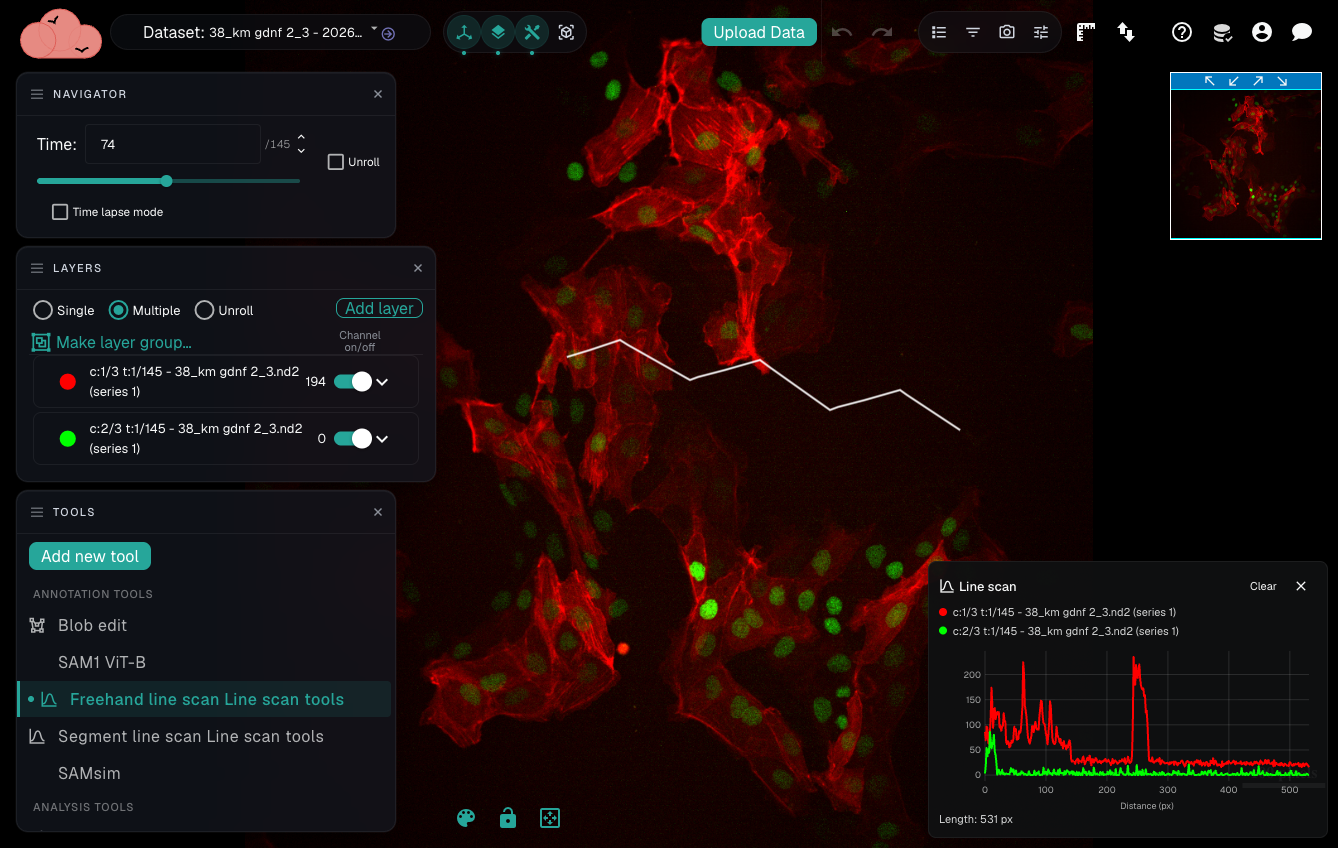
The line scan tool lets you draw a line across your image and immediately see a plot of raw pixel intensity along that line, without creating any stored annotations. This is handy for inspecting signal profiles, comparing channels, checking for colocalization, or locating edges and peaks.

<figure><img src="/files/UqYYS3MniV2lc6Z4J9iV" alt=""><figcaption><p>A freehand line scan across several cells, with the live intensity profile for each channel shown at the bottom right</p></figcaption></figure>

### How to use

1. **Add a line scan tool** from the tool menu. Two variants are available:
   * **Freehand**: Drag to draw a freeform line; the scan completes when you release the mouse.
   * **Segment**: Click once to start and once to end a straight line segment.
2. **Draw across the feature** you want to examine. A panel appears at the bottom right of the viewer showing the intensity profile.
3. The profile updates live as you draw, with one colored trace per channel (matching each layer's color) and a legend. Hover over the plot to read the intensity at a given position.
4. **Close the panel** to dismiss and reset the scan.

### Options

* **Channel selection**: When creating the tool, you can optionally pick a single channel to plot. The panel can then toggle between showing all visible channels and just the selected one.

### Technical details

Intensities are read as raw, unstyled pixel values from the image tiles (not the contrast-adjusted display values) and sampled along the line. The plotted values therefore reflect the true underlying data, making them suitable for quantitative comparison.